Lesson 9: Data Manipulation with dplyr

Author

Gabriel Odom

Published

September 30, 2019

Review

What did we learn last class?

Find some raw data
Reading in flat text / CSV files
Tibbles and “tidy” data
Writing flat text / CSV files
The pipe (%>%) operator

Outline

In this lesson, we will cover the following:

Subset Rows with filter()
Sort Rows with arrange()
Select and Move Columns with select()
Create New Columns with mutate()
Grouping and Group Summaries with group_by() and summarise()
Using *_join() to Merge Tibbles

Reading, Videos, and Assignments

Watch: https://www.youtube.com/playlist?list=PLHKz7LkI0oR2Huix3BcCUJDB_vGchd6NH
Read:
- The “Data Transformation” chapter of R4DS (https://r4ds.hadley.nz/data-transform.html)
- The “Data Tidying” chapter of R4DS (https://r4ds.hadley.nz/data-tidy.html)
- The “Joins” chapter of R4DS (https://r4ds.hadley.nz/joins.html)
Do: complete exercises from the readings

Overview of Common Functions

These functions all operate on tidy data frames:

filter(): return rows that match a certain set of conditions
arrange(): sort rows by a given set of measurements
select(): select, rename, and / or reorder columns
mutate(): create new columns (often as functions of your existing columns)
group_by(): group rows by chosen columns
summarise(): collapse multiple rows into one (often paired with group_by() for group summaries)
*_join(): match observations from one tibble to observations from another

All of these functions have very similar syntax: function(data_df, ...). The ellipsis will take in the additional conditions or arguments for the function, and column names are passed unquoted. Because these functions all take in the data as their first argument and return the new data set, these functions are often written with the pipe operator we learned last class as data_df %>% function(...). Additionally, these functions do not create new data objects. If you want to keep the transformed data table you’ve created, you must store it as an object.

Important

The dplyr functions do not create new data objects. If you want to keep the transformed data table you’ve created, you must store it as an object.

These functions are all from the dplyr package, which is in the tidyverse. Load it now.

library(tidyverse)

If you get stuck, the dplyr cheat sheet is here: https://www.rstudio.com/wp-content/uploads/2015/02/data-wrangling-cheatsheet.pdf

Example Data

Our example data set has measurements on all flights departing the Greater New York City area in 2013. We will use this data set to explore a few of the more commonly-used dplyr functions. Load the nycflights13 package you installed last class:

library(nycflights13)
flights

# A tibble: 336,776 × 19
    year month   day dep_time sched_dep_time dep_delay arr_time sched_arr_time
   <int> <int> <int>    <int>          <int>     <dbl>    <int>          <int>
 1  2013     1     1      517            515         2      830            819
 2  2013     1     1      533            529         4      850            830
 3  2013     1     1      542            540         2      923            850
 4  2013     1     1      544            545        -1     1004           1022
 5  2013     1     1      554            600        -6      812            837
 6  2013     1     1      554            558        -4      740            728
 7  2013     1     1      555            600        -5      913            854
 8  2013     1     1      557            600        -3      709            723
 9  2013     1     1      557            600        -3      838            846
10  2013     1     1      558            600        -2      753            745
# ℹ 336,766 more rows
# ℹ 11 more variables: arr_delay <dbl>, carrier <chr>, flight <int>,
#   tailnum <chr>, origin <chr>, dest <chr>, air_time <dbl>, distance <dbl>,
#   hour <dbl>, minute <dbl>, time_hour <dttm>

This data set has 336,776 unique flights and 19 measurements on those flights.

Subset Rows with `filter()`

The filter function takes in the data frame and a logical argument. Rows that return TRUE for that logical argument are returned as a subset of the original data frame. For example, we would like to inspect only flights that happened on 1 January, 2013.

filter(flights, month == 1, day == 1)

# A tibble: 842 × 19
    year month   day dep_time sched_dep_time dep_delay arr_time sched_arr_time
   <int> <int> <int>    <int>          <int>     <dbl>    <int>          <int>
 1  2013     1     1      517            515         2      830            819
 2  2013     1     1      533            529         4      850            830
 3  2013     1     1      542            540         2      923            850
 4  2013     1     1      544            545        -1     1004           1022
 5  2013     1     1      554            600        -6      812            837
 6  2013     1     1      554            558        -4      740            728
 7  2013     1     1      555            600        -5      913            854
 8  2013     1     1      557            600        -3      709            723
 9  2013     1     1      557            600        -3      838            846
10  2013     1     1      558            600        -2      753            745
# ℹ 832 more rows
# ℹ 11 more variables: arr_delay <dbl>, carrier <chr>, flight <int>,
#   tailnum <chr>, origin <chr>, dest <chr>, air_time <dbl>, distance <dbl>,
#   hour <dbl>, minute <dbl>, time_hour <dttm>

This code selects the 842 rows of the flights data frame where the month column is equal to the number 1 (for January) and the day column is also equal to 1. The equivalent code with the pipe operator from last session is almost exactly the same:

flights %>% filter(month == 1, day == 1)

# A tibble: 842 × 19
    year month   day dep_time sched_dep_time dep_delay arr_time sched_arr_time
   <int> <int> <int>    <int>          <int>     <dbl>    <int>          <int>
 1  2013     1     1      517            515         2      830            819
 2  2013     1     1      533            529         4      850            830
 3  2013     1     1      542            540         2      923            850
 4  2013     1     1      544            545        -1     1004           1022
 5  2013     1     1      554            600        -6      812            837
 6  2013     1     1      554            558        -4      740            728
 7  2013     1     1      555            600        -5      913            854
 8  2013     1     1      557            600        -3      709            723
 9  2013     1     1      557            600        -3      838            846
10  2013     1     1      558            600        -2      753            745
# ℹ 832 more rows
# ℹ 11 more variables: arr_delay <dbl>, carrier <chr>, flight <int>,
#   tailnum <chr>, origin <chr>, dest <chr>, air_time <dbl>, distance <dbl>,
#   hour <dbl>, minute <dbl>, time_hour <dttm>

As a review, the pipe turns x %>% f(y) into f(x, y). Pipes allow us to read code from left-to-right and top-to-bottom, rather than inside out with a giant nest of parentheses.

Examples

For these examples, we need to read the documentation on the flights data first. Make sure you know what the columns are and their values.

Find all the flights on Christmas Eve. We’ll use the same code structure as the code for finding all the New Year’s Day flights.

flights %>% filter(month == 12, day == 24)

# A tibble: 761 × 19
    year month   day dep_time sched_dep_time dep_delay arr_time sched_arr_time
   <int> <int> <int>    <int>          <int>     <dbl>    <int>          <int>
 1  2013    12    24        9           2359        10      444            445
 2  2013    12    24      458            500        -2      652            651
 3  2013    12    24      513            515        -2      813            814
 4  2013    12    24      543            540         3      844            850
 5  2013    12    24      546            550        -4     1032           1027
 6  2013    12    24      555            600        -5      851            915
 7  2013    12    24      556            600        -4      845            846
 8  2013    12    24      557            600        -3      908            849
 9  2013    12    24      558            600        -2      827            831
10  2013    12    24      558            600        -2      729            718
# ℹ 751 more rows
# ℹ 11 more variables: arr_delay <dbl>, carrier <chr>, flight <int>,
#   tailnum <chr>, origin <chr>, dest <chr>, air_time <dbl>, distance <dbl>,
#   hour <dbl>, minute <dbl>, time_hour <dttm>

Find all flights during the summer months (June, July, and August).

flights %>% filter(month %in% c(6, 7, 8))

# A tibble: 86,995 × 19
    year month   day dep_time sched_dep_time dep_delay arr_time sched_arr_time
   <int> <int> <int>    <int>          <int>     <dbl>    <int>          <int>
 1  2013     6     1        2           2359         3      341            350
 2  2013     6     1      451            500        -9      624            640
 3  2013     6     1      506            515        -9      715            800
 4  2013     6     1      534            545       -11      800            829
 5  2013     6     1      538            545        -7      925            922
 6  2013     6     1      539            540        -1      832            840
 7  2013     6     1      546            600       -14      850            910
 8  2013     6     1      551            600        -9      828            850
 9  2013     6     1      552            600        -8      647            655
10  2013     6     1      553            600        -7      700            711
# ℹ 86,985 more rows
# ℹ 11 more variables: arr_delay <dbl>, carrier <chr>, flight <int>,
#   tailnum <chr>, origin <chr>, dest <chr>, air_time <dbl>, distance <dbl>,
#   hour <dbl>, minute <dbl>, time_hour <dttm>

Find all flights that did not depart from Newark Liberty.

flights %>% filter(origin != "EWR")

# A tibble: 215,941 × 19
    year month   day dep_time sched_dep_time dep_delay arr_time sched_arr_time
   <int> <int> <int>    <int>          <int>     <dbl>    <int>          <int>
 1  2013     1     1      533            529         4      850            830
 2  2013     1     1      542            540         2      923            850
 3  2013     1     1      544            545        -1     1004           1022
 4  2013     1     1      554            600        -6      812            837
 5  2013     1     1      557            600        -3      709            723
 6  2013     1     1      557            600        -3      838            846
 7  2013     1     1      558            600        -2      753            745
 8  2013     1     1      558            600        -2      849            851
 9  2013     1     1      558            600        -2      853            856
10  2013     1     1      558            600        -2      924            917
# ℹ 215,931 more rows
# ℹ 11 more variables: arr_delay <dbl>, carrier <chr>, flight <int>,
#   tailnum <chr>, origin <chr>, dest <chr>, air_time <dbl>, distance <dbl>,
#   hour <dbl>, minute <dbl>, time_hour <dttm>

Find all JetBlue (“B6”) or Southwest (“WN”) flights.

flights %>% filter(carrier == "B6" | carrier == "WN")

# A tibble: 66,910 × 19
    year month   day dep_time sched_dep_time dep_delay arr_time sched_arr_time
   <int> <int> <int>    <int>          <int>     <dbl>    <int>          <int>
 1  2013     1     1      544            545        -1     1004           1022
 2  2013     1     1      555            600        -5      913            854
 3  2013     1     1      557            600        -3      838            846
 4  2013     1     1      558            600        -2      849            851
 5  2013     1     1      558            600        -2      853            856
 6  2013     1     1      559            559         0      702            706
 7  2013     1     1      600            600         0      851            858
 8  2013     1     1      601            600         1      844            850
 9  2013     1     1      613            610         3      925            921
10  2013     1     1      615            615         0     1039           1100
# ℹ 66,900 more rows
# ℹ 11 more variables: arr_delay <dbl>, carrier <chr>, flight <int>,
#   tailnum <chr>, origin <chr>, dest <chr>, air_time <dbl>, distance <dbl>,
#   hour <dbl>, minute <dbl>, time_hour <dttm>

Find any flights out of LaGuardia that actually left on time.

flights %>% filter(origin == "LGA" & dep_delay <= 0)

# A tibble: 67,819 × 19
    year month   day dep_time sched_dep_time dep_delay arr_time sched_arr_time
   <int> <int> <int>    <int>          <int>     <dbl>    <int>          <int>
 1  2013     1     1      554            600        -6      812            837
 2  2013     1     1      557            600        -3      709            723
 3  2013     1     1      558            600        -2      753            745
 4  2013     1     1      559            600        -1      941            910
 5  2013     1     1      600            600         0      851            858
 6  2013     1     1      600            600         0      837            825
 7  2013     1     1      602            610        -8      812            820
 8  2013     1     1      602            605        -3      821            805
 9  2013     1     1      623            627        -4      933            932
10  2013     1     1      624            630        -6      840            830
# ℹ 67,809 more rows
# ℹ 11 more variables: arr_delay <dbl>, carrier <chr>, flight <int>,
#   tailnum <chr>, origin <chr>, dest <chr>, air_time <dbl>, distance <dbl>,
#   hour <dbl>, minute <dbl>, time_hour <dttm>

Sort Rows with `arrange()`

The arrange() function takes in a data frame and a set of columns to sort on. We can sort the flights by in increasing order by the day of the year: we sort by month, then by day within month.

flights %>% arrange(year, month, day)

# A tibble: 336,776 × 19
    year month   day dep_time sched_dep_time dep_delay arr_time sched_arr_time
   <int> <int> <int>    <int>          <int>     <dbl>    <int>          <int>
 1  2013     1     1      517            515         2      830            819
 2  2013     1     1      533            529         4      850            830
 3  2013     1     1      542            540         2      923            850
 4  2013     1     1      544            545        -1     1004           1022
 5  2013     1     1      554            600        -6      812            837
 6  2013     1     1      554            558        -4      740            728
 7  2013     1     1      555            600        -5      913            854
 8  2013     1     1      557            600        -3      709            723
 9  2013     1     1      557            600        -3      838            846
10  2013     1     1      558            600        -2      753            745
# ℹ 336,766 more rows
# ℹ 11 more variables: arr_delay <dbl>, carrier <chr>, flight <int>,
#   tailnum <chr>, origin <chr>, dest <chr>, air_time <dbl>, distance <dbl>,
#   hour <dbl>, minute <dbl>, time_hour <dttm>

Also, we can sort the flights by departure delay time.

flights %>% arrange(desc(dep_delay))

# A tibble: 336,776 × 19
    year month   day dep_time sched_dep_time dep_delay arr_time sched_arr_time
   <int> <int> <int>    <int>          <int>     <dbl>    <int>          <int>
 1  2013     1     9      641            900      1301     1242           1530
 2  2013     6    15     1432           1935      1137     1607           2120
 3  2013     1    10     1121           1635      1126     1239           1810
 4  2013     9    20     1139           1845      1014     1457           2210
 5  2013     7    22      845           1600      1005     1044           1815
 6  2013     4    10     1100           1900       960     1342           2211
 7  2013     3    17     2321            810       911      135           1020
 8  2013     6    27      959           1900       899     1236           2226
 9  2013     7    22     2257            759       898      121           1026
10  2013    12     5      756           1700       896     1058           2020
# ℹ 336,766 more rows
# ℹ 11 more variables: arr_delay <dbl>, carrier <chr>, flight <int>,
#   tailnum <chr>, origin <chr>, dest <chr>, air_time <dbl>, distance <dbl>,
#   hour <dbl>, minute <dbl>, time_hour <dttm>

Further, we can combine this with the filter() commmand to sort the American Airlines flights out of JFK on the day before Thanksgiving by their duration. By the way, see how easy it is to chain rather complicated commands together? You might begin to imagine that we are only scratching the surface of what we can do with dplyr…

flights %>%
  filter(carrier == "AA") %>% 
  filter(origin == "JFK") %>% 
  filter(month == 11) %>% 
  filter(day == 27) %>%
  arrange(desc(air_time))

# A tibble: 37 × 19
    year month   day dep_time sched_dep_time dep_delay arr_time sched_arr_time
   <int> <int> <int>    <int>          <int>     <dbl>    <int>          <int>
 1  2013    11    27     1529           1530        -1     1903           1915
 2  2013    11    27      805            800         5     1129           1135
 3  2013    11    27     1740           1745        -5     2103           2125
 4  2013    11    27     1022           1030        -8     1319           1355
 5  2013    11    27      724            730        -6     1058           1050
 6  2013    11    27     1340           1345        -5     1648           1705
 7  2013    11    27     1543           1545        -2     1845           1920
 8  2013    11    27     1849           1850        -1     2209           2220
 9  2013    11    27     1900           1900         0     2229           2215
10  2013    11    27     1141            900       161     1429           1225
# ℹ 27 more rows
# ℹ 11 more variables: arr_delay <dbl>, carrier <chr>, flight <int>,
#   tailnum <chr>, origin <chr>, dest <chr>, air_time <dbl>, distance <dbl>,
#   hour <dbl>, minute <dbl>, time_hour <dttm>

As an aside, look how clean this code looks because of our pipes! Imagine trying to write this as a set of nested functions. Not pretty.

Select and Move Columns with `select()`

While filter() and arrange() help us select and sort individual observations (rows), the select() function helps us select, rename, or reorder the measurements (columns) of a data frame.

Select Columns that Meet Our Criteria

We first select three columns specifically by their names.

flights %>% select(year, month, day)

# A tibble: 336,776 × 3
    year month   day
   <int> <int> <int>
 1  2013     1     1
 2  2013     1     1
 3  2013     1     1
 4  2013     1     1
 5  2013     1     1
 6  2013     1     1
 7  2013     1     1
 8  2013     1     1
 9  2013     1     1
10  2013     1     1
# ℹ 336,766 more rows

Notice that we only have the three columns we explicitly requested by name and no more. The select() function will drop whatever we don’t ask for by default, but we can change this behaviour by adding the additional everything() argument (we’ll come back to this in the “reordering columns” section).

We could have also specified a range of column names to achieve the same effect.

flights %>% select(year:day)

# A tibble: 336,776 × 3
    year month   day
   <int> <int> <int>
 1  2013     1     1
 2  2013     1     1
 3  2013     1     1
 4  2013     1     1
 5  2013     1     1
 6  2013     1     1
 7  2013     1     1
 8  2013     1     1
 9  2013     1     1
10  2013     1     1
# ℹ 336,766 more rows

If you have used regular expressions or performed string manipulation before, you can also use the following modifiers to the select() function:

Find all the columns with names starting with “dep_”.

flights %>% select(starts_with("dep_"))

# A tibble: 336,776 × 2
   dep_time dep_delay
      <int>     <dbl>
 1      517         2
 2      533         4
 3      542         2
 4      544        -1
 5      554        -6
 6      554        -4
 7      555        -5
 8      557        -3
 9      557        -3
10      558        -2
# ℹ 336,766 more rows

Find all the columns with names ending with “ay”.

flights %>% select(ends_with("ay"))

# A tibble: 336,776 × 3
     day dep_delay arr_delay
   <int>     <dbl>     <dbl>
 1     1         2        11
 2     1         4        20
 3     1         2        33
 4     1        -1       -18
 5     1        -6       -25
 6     1        -4        12
 7     1        -5        19
 8     1        -3       -14
 9     1        -3        -8
10     1        -2         8
# ℹ 336,766 more rows

Find all the columns with names that contain “time”.

flights %>% select(contains("time"))

# A tibble: 336,776 × 6
   dep_time sched_dep_time arr_time sched_arr_time air_time time_hour          
      <int>          <int>    <int>          <int>    <dbl> <dttm>             
 1      517            515      830            819      227 2013-01-01 05:00:00
 2      533            529      850            830      227 2013-01-01 05:00:00
 3      542            540      923            850      160 2013-01-01 05:00:00
 4      544            545     1004           1022      183 2013-01-01 05:00:00
 5      554            600      812            837      116 2013-01-01 06:00:00
 6      554            558      740            728      150 2013-01-01 05:00:00
 7      555            600      913            854      158 2013-01-01 06:00:00
 8      557            600      709            723       53 2013-01-01 06:00:00
 9      557            600      838            846      140 2013-01-01 06:00:00
10      558            600      753            745      138 2013-01-01 06:00:00
# ℹ 336,766 more rows

Find all the columns with names that start with exactly three lower case letters followed by “_“.

flights %>% select(matches("^[a-z]{3}\\_"))

# A tibble: 336,776 × 5
   dep_time dep_delay arr_time arr_delay air_time
      <int>     <dbl>    <int>     <dbl>    <dbl>
 1      517         2      830        11      227
 2      533         4      850        20      227
 3      542         2      923        33      160
 4      544        -1     1004       -18      183
 5      554        -6      812       -25      116
 6      554        -4      740        12      150
 7      555        -5      913        19      158
 8      557        -3      709       -14       53
 9      557        -3      838        -8      140
10      558        -2      753         8      138
# ℹ 336,766 more rows

The matches() function takes in a regular expression. If you have never used regular expressions for string queries before, don’t be afraid. You can do most of the things you need without ever touching the matches() function. However, if you do find yourself needing some help with string manipulation in R, please see the stringr package cheat sheet from the RStudio Cheat Sheets page and the strings chapter from R for Data Science. You can also practice building expressions on https://regexr.com/. We will also learn a bit more about the stringr package in a later lesson.

Remove, Reorder, or Rename

Remove Columns

We can also use “negative indexing” to select all the columns except for the columns we named.

flights %>% select(-(year:day))

# A tibble: 336,776 × 16
   dep_time sched_dep_time dep_delay arr_time sched_arr_time arr_delay carrier
      <int>          <int>     <dbl>    <int>          <int>     <dbl> <chr>  
 1      517            515         2      830            819        11 UA     
 2      533            529         4      850            830        20 UA     
 3      542            540         2      923            850        33 AA     
 4      544            545        -1     1004           1022       -18 B6     
 5      554            600        -6      812            837       -25 DL     
 6      554            558        -4      740            728        12 UA     
 7      555            600        -5      913            854        19 B6     
 8      557            600        -3      709            723       -14 EV     
 9      557            600        -3      838            846        -8 B6     
10      558            600        -2      753            745         8 AA     
# ℹ 336,766 more rows
# ℹ 9 more variables: flight <int>, tailnum <chr>, origin <chr>, dest <chr>,
#   air_time <dbl>, distance <dbl>, hour <dbl>, minute <dbl>, time_hour <dttm>

This is particularly useful when we have filtered out all of one type of observation. We can then remove the redundant column information. For instance, previously we filtered only the flights leaving on 1 January, 2013. However, we still had the year, month, and day columns in this data table, even though this information was superfluous after filtering.

# Before
flights %>%
  filter(month == 1, day == 1)

# A tibble: 842 × 19
    year month   day dep_time sched_dep_time dep_delay arr_time sched_arr_time
   <int> <int> <int>    <int>          <int>     <dbl>    <int>          <int>
 1  2013     1     1      517            515         2      830            819
 2  2013     1     1      533            529         4      850            830
 3  2013     1     1      542            540         2      923            850
 4  2013     1     1      544            545        -1     1004           1022
 5  2013     1     1      554            600        -6      812            837
 6  2013     1     1      554            558        -4      740            728
 7  2013     1     1      555            600        -5      913            854
 8  2013     1     1      557            600        -3      709            723
 9  2013     1     1      557            600        -3      838            846
10  2013     1     1      558            600        -2      753            745
# ℹ 832 more rows
# ℹ 11 more variables: arr_delay <dbl>, carrier <chr>, flight <int>,
#   tailnum <chr>, origin <chr>, dest <chr>, air_time <dbl>, distance <dbl>,
#   hour <dbl>, minute <dbl>, time_hour <dttm>

# After
flights %>%
  filter(month == 1, day == 1) %>% 
  select(-year, -month, -day)

# A tibble: 842 × 16
   dep_time sched_dep_time dep_delay arr_time sched_arr_time arr_delay carrier
      <int>          <int>     <dbl>    <int>          <int>     <dbl> <chr>  
 1      517            515         2      830            819        11 UA     
 2      533            529         4      850            830        20 UA     
 3      542            540         2      923            850        33 AA     
 4      544            545        -1     1004           1022       -18 B6     
 5      554            600        -6      812            837       -25 DL     
 6      554            558        -4      740            728        12 UA     
 7      555            600        -5      913            854        19 B6     
 8      557            600        -3      709            723       -14 EV     
 9      557            600        -3      838            846        -8 B6     
10      558            600        -2      753            745         8 AA     
# ℹ 832 more rows
# ℹ 9 more variables: flight <int>, tailnum <chr>, origin <chr>, dest <chr>,
#   air_time <dbl>, distance <dbl>, hour <dbl>, minute <dbl>, time_hour <dttm>

Reorder Columns

As we alluded to above, we can also use the select() function to change the order of the columns of the data table, without removing the columns we don’t explicitely name, with the helpof the everything() function.

flights %>% select(time_hour, air_time, everything())

# A tibble: 336,776 × 19
   time_hour           air_time  year month   day dep_time sched_dep_time
   <dttm>                 <dbl> <int> <int> <int>    <int>          <int>
 1 2013-01-01 05:00:00      227  2013     1     1      517            515
 2 2013-01-01 05:00:00      227  2013     1     1      533            529
 3 2013-01-01 05:00:00      160  2013     1     1      542            540
 4 2013-01-01 05:00:00      183  2013     1     1      544            545
 5 2013-01-01 06:00:00      116  2013     1     1      554            600
 6 2013-01-01 05:00:00      150  2013     1     1      554            558
 7 2013-01-01 06:00:00      158  2013     1     1      555            600
 8 2013-01-01 06:00:00       53  2013     1     1      557            600
 9 2013-01-01 06:00:00      140  2013     1     1      557            600
10 2013-01-01 06:00:00      138  2013     1     1      558            600
# ℹ 336,766 more rows
# ℹ 12 more variables: dep_delay <dbl>, arr_time <int>, sched_arr_time <int>,
#   arr_delay <dbl>, carrier <chr>, flight <int>, tailnum <chr>, origin <chr>,
#   dest <chr>, distance <dbl>, hour <dbl>, minute <dbl>

Rename Columns

While the select() function can rename columns, we recommend using the rename() function for better readibility of your code instead. This function takes in the data table and an argument that follows the [new name] = [old name] syntax. For example, we notice that all of the column names with more than one word are written in snake_case except for tailnum. We can rename this column to match our naming convention. However, we must save the results of the output of the rename() function. Otherwise, the data table with the new column name will print to the screen but never be saved anywhere. We can use the names() function to check that our new name stuck.

flights <- rename(flights, tail_num = tailnum)
names(flights)

 [1] "year"           "month"          "day"            "dep_time"      
 [5] "sched_dep_time" "dep_delay"      "arr_time"       "sched_arr_time"
 [9] "arr_delay"      "carrier"        "flight"         "tail_num"      
[13] "origin"         "dest"           "air_time"       "distance"      
[17] "hour"           "minute"         "time_hour"

Overwriting Data

Note that I am saving the old data set as a new data set with the same name. Only do this if you are positive that you don’t want to “go back a step”. This action cannot be undone. While you are learning, I always recommend that you save new objects with new names.

Create New Columns with `mutate()`

Up to this point, we have only teased out observational or measurement information that was already in the data table. But what if we want to create a new measurement as a function of some existing measurements? We can do so with the mutate() function. This function’s syntax is very similar to the syntax of the rename() function: the data frame is first, then [new column name] = {expression}.

For example, we will find all the continental US flights with the strongest potential jet stream delay (the West Coast airports). We would like to find the land speed of each of these flights and add it to our smaller data table.

westCoast <- c(
  "BUR", "HNL", "LAS", "LAX", "OAK", "PDX", "PHX", "PSP", "RNO", "SAN", "SEA",
  "SFO", "SJC", "SLC"
)

jetStreamFlights <- flights %>% 
  filter(dest %in% westCoast) %>% 
  select(month, day, dest, ends_with("delay"), distance, air_time)

jetStreamFlights %>% 
  mutate(speed_mph = distance / (air_time / 60))

# A tibble: 52,377 × 8
   month   day dest  dep_delay arr_delay distance air_time speed_mph
   <int> <int> <chr>     <dbl>     <dbl>    <dbl>    <dbl>     <dbl>
 1     1     1 LAX          -2         7     2475      345      430.
 2     1     1 SFO          -2       -14     2565      361      426.
 3     1     1 LAS          -1        -8     2227      337      396.
 4     1     1 SFO          11        14     2586      366      424.
 5     1     1 PHX          -8         3     2133      342      374.
 6     1     1 PHX          -3         0     2153      330      391.
 7     1     1 LAX          -2        29     2454      366      402.
 8     1     1 LAS          -4        -6     2248      323      418.
 9     1     1 SLC           0        -9     1990      294      406.
10     1     1 SFO          -5        -8     2586      362      429.
# ℹ 52,367 more rows

If we only care about the speeds themselves, we can select the speed_mph column we just created.

jetStreamFlights %>% 
  mutate(speed_mph = distance / (air_time / 60)) %>% 
  select(speed_mph)

# A tibble: 52,377 × 1
   speed_mph
       <dbl>
 1      430.
 2      426.
 3      396.
 4      424.
 5      374.
 6      391.
 7      402.
 8      418.
 9      406.
10      429.
# ℹ 52,367 more rows

Alternatively, if we only care about the one column we are creating with mutate(), then we add the argument .keep = "none". This operation is shorthand for mutate(newCol = <calculation>) then select(newCol).

jetStreamFlights %>% 
  mutate(speed_mph = distance / (air_time / 60), .keep = "none")

# A tibble: 52,377 × 1
   speed_mph
       <dbl>
 1      430.
 2      426.
 3      396.
 4      424.
 5      374.
 6      391.
 7      402.
 8      418.
 9      406.
10      429.
# ℹ 52,367 more rows

The transmute() Function

This operation, mutate() then select(), used to have it’s own function, called transmute(). I would teach it, but it rarely every came up in practice. This function has now been replaced (technically “superseded”) by adding an option to the .keep argument of mutate(), which is—in my opinion—much better.

The `case_when()` Function

We can use the mutate() in conjunction with the case_when() function to add a label indicating if the flight has beverage service, meals for sale, or meals included. In order to use the case_when() function, we need to map out all of the meal options and the flight durations that trigger them. This will take the form of a giant IF-THEN ladder:

IF air_time <= 50 THEN no beverage service or snacks
IF 50 < air_time AND air_time <= 2.5 * 60 THEN beverage and snacks
IF 2.5 * 60 < air_time AND air_time <= 4 * 60 THEN beverage and snacks with meals for sale
IF 4 * 60 < air_time AND air_time <= 7 * 60 THEN beverage, snacks, and 1 meal
IF 7 * 60 < air_time THEN beverage, snacks, and 2 meals

The syntax to use the case_when() function is:

the IF statement is automatically included
AND and OR use R’s regular functions: &, |
THEN is the tilde symbol, ~.

Thus, the code to add flight food labels is:

flights %>%
  mutate(
    food = case_when(
      air_time <= 50 ~
        "none",
      50 < air_time & air_time <= 2.5 * 60 ~
        "drinks + light snacks",
      2.5 * 60 < air_time & air_time <= 4 * 60 ~
        "drinks + heavy snacks",
      4 * 60 < air_time & air_time <= 7 * 60 ~
        "drinks, snacks, and 1 meal",
      7 * 60 < air_time ~
        "drinks, snacks, and 2 meals"
    )
  ) %>%  
  select(air_time, food)

# A tibble: 336,776 × 2
   air_time food                 
      <dbl> <chr>                
 1      227 drinks + heavy snacks
 2      227 drinks + heavy snacks
 3      160 drinks + heavy snacks
 4      183 drinks + heavy snacks
 5      116 drinks + light snacks
 6      150 drinks + light snacks
 7      158 drinks + heavy snacks
 8       53 drinks + light snacks
 9      140 drinks + light snacks
10      138 drinks + light snacks
# ℹ 336,766 more rows

The code pieces on the left and right of the tilde are called expressions, and they are used to construct functions. The mutate() function can also make use of functions you construct. We will discuss this more in the lesson on control flow and functions.

Examples

The possible uses of the mutate() function are practically endless, but we can look a few examples.

Basic Arithmetic

We may not be concerned with the actual distance of a flight, but perhaps its difference from the average flight distance.

flights %>% 
  mutate(residual_dist = distance - mean(distance), .keep = "none")

# A tibble: 336,776 × 1
   residual_dist
           <dbl>
 1         360. 
 2         376. 
 3          49.1
 4         536. 
 5        -278. 
 6        -321. 
 7          25.1
 8        -811. 
 9         -95.9
10        -307. 
# ℹ 336,766 more rows

Perhaps we want to add an indicator for “long flights” (American Airlines considers a long flight any flight over four-and-a-half hours) and then order these flights by flight time, excluding flights to Honolulu.

flights %>%
  mutate(long_flight = air_time >= 270) %>% 
  filter(dest != "HNL") %>% 
  select(dest, long_flight, air_time, everything()) %>% 
  arrange(desc(air_time))

# A tibble: 336,069 × 20
   dest  long_flight air_time  year month   day dep_time sched_dep_time
   <chr> <lgl>          <dbl> <int> <int> <int>    <int>          <int>
 1 SFO   TRUE             490  2013     7    28     1727           1730
 2 LAX   TRUE             440  2013    11    22     1812           1815
 3 SFO   TRUE             438  2013    12     6     1727           1730
 4 ANC   TRUE             434  2013     8     3     1615           1615
 5 ANC   TRUE             428  2013     8    24     1633           1625
 6 SFO   TRUE             426  2013    12     6     1746           1745
 7 SFO   TRUE             422  2013     2     4      747            745
 8 LAX   TRUE             422  2013     7    10     1814           1815
 9 SFO   TRUE             421  2013     8     8     1724           1710
10 SFO   TRUE             420  2013     8     8     1819           1519
# ℹ 336,059 more rows
# ℹ 12 more variables: dep_delay <dbl>, arr_time <int>, sched_arr_time <int>,
#   arr_delay <dbl>, carrier <chr>, flight <int>, tail_num <chr>, origin <chr>,
#   distance <dbl>, hour <dbl>, minute <dbl>, time_hour <dttm>

Time and Modular Arithmetic (Optional)

The departure and arrival times are presented in a readable form of hours as the first two digits and and minutes as the last two (for example, 5:17AM is 517). However, we can’t subtract arrival time from departure time because these times are not proper continuous variables. We can create two new columns which measure the number of minutes after midnight for both departure and arrival (using modular arithmetic). We will then move these columns to the front so we can see them.

flights %>%
  mutate(
    dep_time_min = (dep_time %/% 100) * 60 + dep_time %% 100,
    arr_time_min = (arr_time %/% 100) * 60 + arr_time %% 100
  ) %>% 
  select(starts_with("dep_time"), starts_with("arr_time"), everything())

# A tibble: 336,776 × 21
   dep_time dep_time_min arr_time arr_time_min  year month   day sched_dep_time
      <int>        <dbl>    <int>        <dbl> <int> <int> <int>          <int>
 1      517          317      830          510  2013     1     1            515
 2      533          333      850          530  2013     1     1            529
 3      542          342      923          563  2013     1     1            540
 4      544          344     1004          604  2013     1     1            545
 5      554          354      812          492  2013     1     1            600
 6      554          354      740          460  2013     1     1            558
 7      555          355      913          553  2013     1     1            600
 8      557          357      709          429  2013     1     1            600
 9      557          357      838          518  2013     1     1            600
10      558          358      753          473  2013     1     1            600
# ℹ 336,766 more rows
# ℹ 13 more variables: dep_delay <dbl>, sched_arr_time <int>, arr_delay <dbl>,
#   carrier <chr>, flight <int>, tail_num <chr>, origin <chr>, dest <chr>,
#   air_time <dbl>, distance <dbl>, hour <dbl>, minute <dbl>, time_hour <dttm>

The %% operator is the modulo operator (sometimes called the “remainder” operator) in R. The a %% b operation returns the remainder after dividing a by b. The %/% operator is the integer division operator; the a %/% b operation returns the quotient of a and b with any decimal information discarded.

Grouping and Group Summaries with `group_by()` and `summarise()`

The summarise() function is very powerful and very flexible. We will not have time to discuss all it can do. For a more complete discussion, see the summarise() section of R for Data Science, chapter 5 (in the 1st edition, chapter 3 in the 2nd edition).

The syntax of summarise() is similar to the mutate() syntax. We can find the average delay of all flights leaving the New York City area in 2013. Because NAs are contagious, we remove them from the calculation with na.rm = TRUE.

flights %>% summarise(delay = mean(dep_delay, na.rm = TRUE))

# A tibble: 1 × 1
  delay
  <dbl>
1  12.6

Incidentally, the NAs are from cancelled flights. We can remove the cancelled flights and save this data set.

not_cancelled <- flights %>% 
  filter(!is.na(dep_delay)) %>% 
  filter(!is.na(arr_delay))

We can also find the arrival delay by destination with group_by(), then check if any cites seem to have less arrival delays (possibly due to changes in wind resistance or traffic control at those airports?).

not_cancelled %>% 
  group_by(dest) %>% 
  summarise(delay = mean(arr_delay)) %>% 
  mutate(resid_delay = delay - mean(delay)) %>% 
  arrange(resid_delay)

# A tibble: 104 × 3
   dest     delay resid_delay
   <chr>    <dbl>       <dbl>
 1 LEX   -22           -30.7 
 2 PSP   -12.7         -21.5 
 3 SNA    -7.87        -16.6 
 4 STT    -3.84        -12.6 
 5 ANC    -2.5         -11.2 
 6 HNL    -1.37        -10.1 
 7 SEA    -1.10         -9.83
 8 MVY    -0.286        -9.02
 9 LGB    -0.0620       -8.79
10 SLC     0.176        -8.56
# ℹ 94 more rows

We can always ungroup our data table with the ungroup() function.

Using the .by Argument

Note that the summarize() and mutate() functions also accept a .by argument, which allows you to specify the grouping for the calculation within the function call. When using the group_by() function, the groups you specify will persist, potentially even after your calculation has been completed. However, when using the .by argument, the groups will NOT persist: they will only be used to execute the computation from the function that called for them. For more discussion on these two options and their differences, see this documentation page on group_by() vs. .by.

Chaining Operations Together

We have already used the pipe (%>%) operator quite a bit. This allows us to chain multiple steps together. For example, we might want to plot the relationship between flight distance and arrival delay (if you don’t remember how to use ggplot(), look back a few lessons).

# Create a "delays" data table
delays <- flights %>% 
  group_by(dest) %>% 
  summarise(
    count = n(),
    dist = mean(distance, na.rm = TRUE),
    delay = mean(arr_delay, na.rm = TRUE)
  ) %>% 
  # We don't want any small airports, or Honolulu
  filter(count > 20, dest != "HNL")

# Plot the delays and add a smoother
ggplot(data = delays) +
  aes(x = dist, y = delay) +
  geom_point(aes(size = count), alpha = 1/3) +
  geom_smooth(se = FALSE)

`geom_smooth()` using method = 'loess' and formula = 'y ~ x'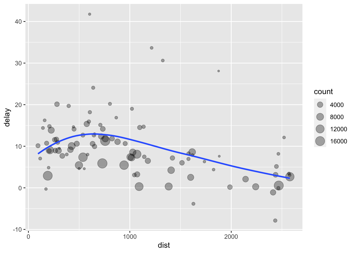

Adding and Visualising Counts

Let’s look at the average delay by plane.

delays <- not_cancelled %>% 
  group_by(tail_num) %>% 
  summarise(
    delay = mean(arr_delay)
  )

ggplot(data = delays) + 
  aes(x = delay) +
  geom_freqpoly(binwidth = 10)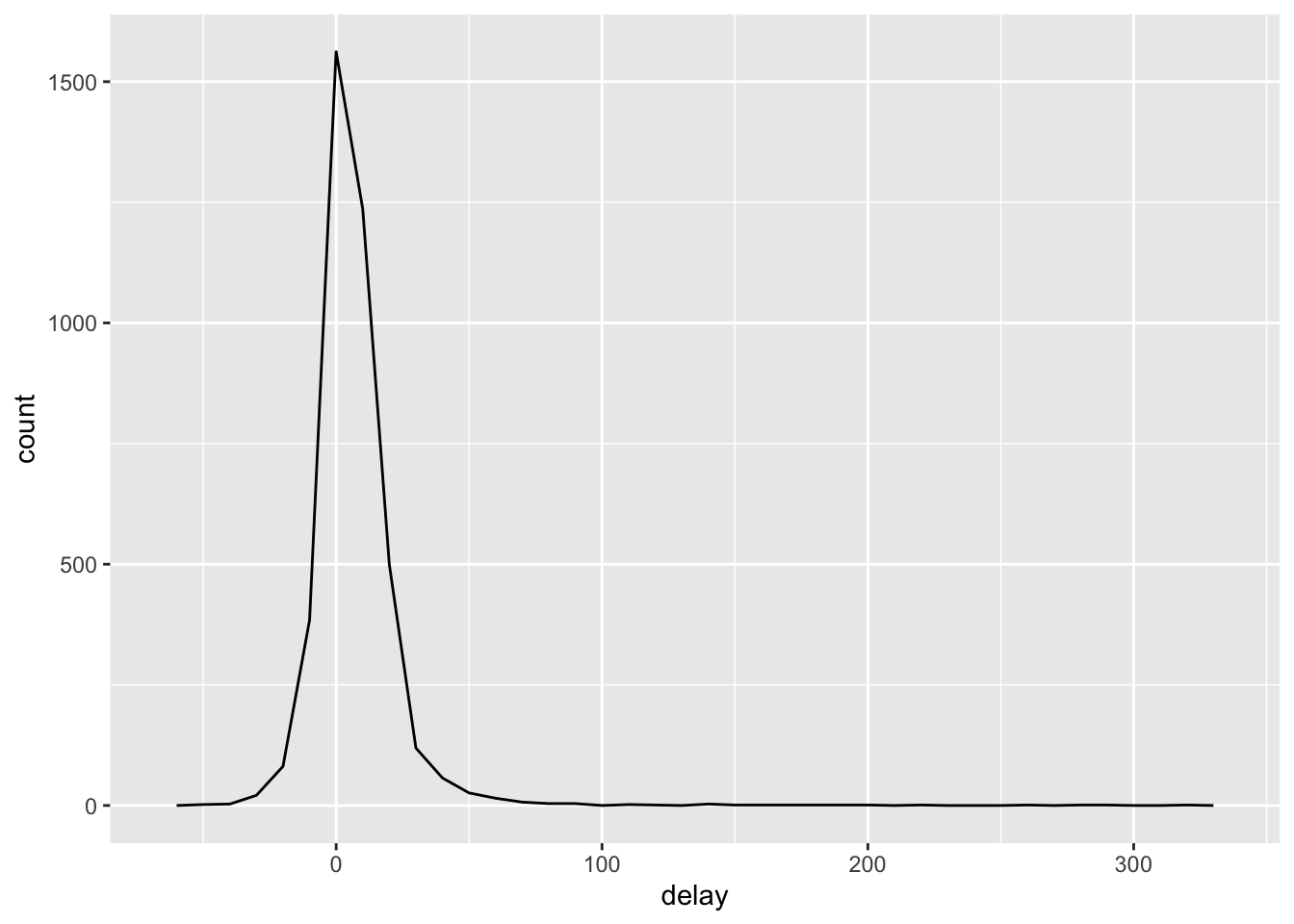

Based on this graph, there are some planes with an average delay of over five hours! But how many flights did that plane make? We need to add a count. Now that we add a count and re-plot the average arrival delay, we immediately see the Central Limit Theorem in action. All those planes with massive average delays only had one or two flights.

delays <- not_cancelled %>% 
  group_by(tail_num) %>% 
  summarise(
    delay = mean(arr_delay, na.rm = TRUE),
    n = n()
  )

ggplot(data = delays) + 
  aes(x = n, y = delay) +
  geom_point(alpha = 1/10)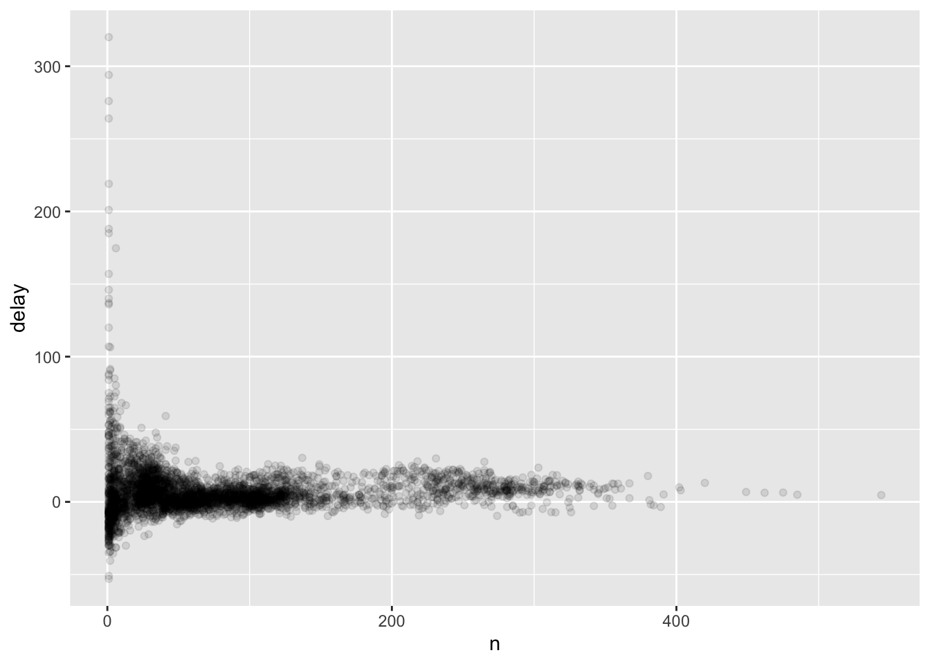

We can remove any planes with fewer than 30 flights and re-visualize the relationships between average delay and number of flights and the overall count-delay distribution.

delays %>% 
  filter(n >= 30) %>% 
  ggplot() + 
    aes(x = n, y = delay) +
    geom_point(alpha = 1/10)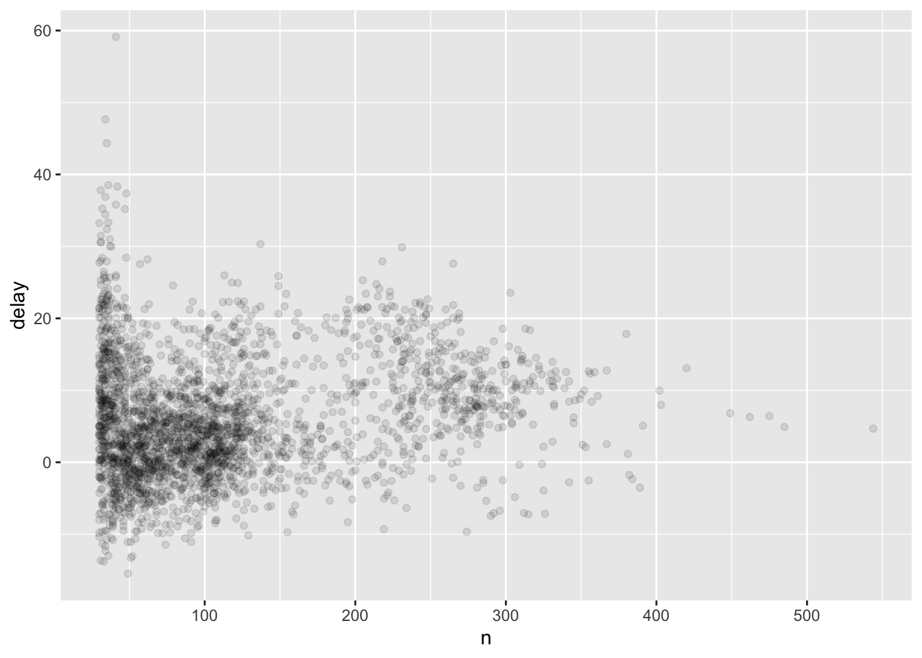

delays %>% 
  filter(n >= 30) %>% 
  ggplot() + 
    aes(x = delay) +
    geom_freqpoly(binwidth = 10)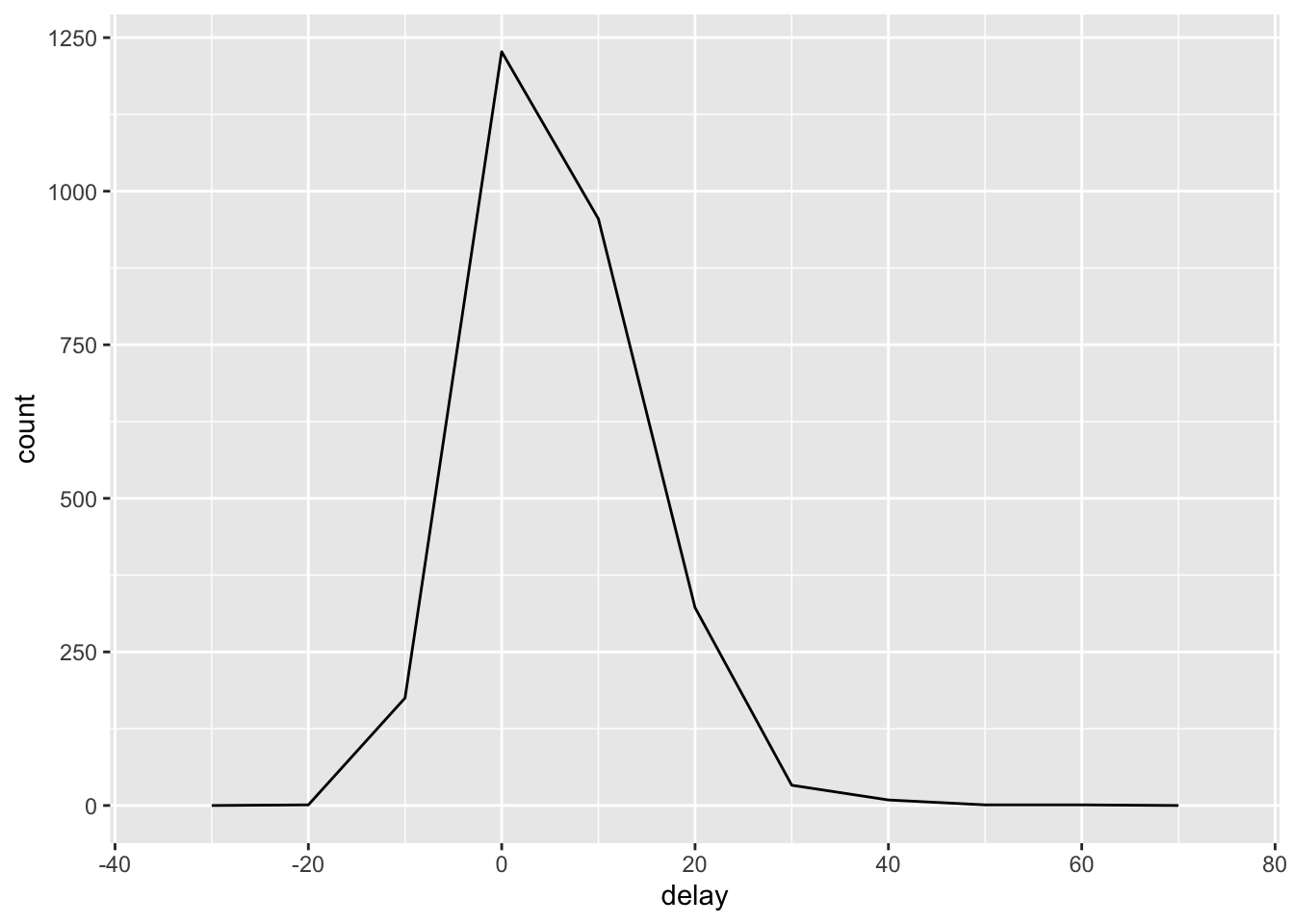

Other Useful Summaries

We know that passengers don’t usually complain if their flight is early, but our dep_delay has negative values for flights which left early. We can find the average true “delay” by taking the summary of only the positive delay values.

not_cancelled %>% 
  group_by(year, month, day) %>% 
  summarise(
    avg_delay1 = mean(arr_delay),
    # the average positive delay
    avg_delay2 = mean(arr_delay[arr_delay > 0])
  )

`summarise()` has grouped output by 'year', 'month'. You can override using the
`.groups` argument.

# A tibble: 365 × 5
# Groups:   year, month [12]
    year month   day avg_delay1 avg_delay2
   <int> <int> <int>      <dbl>      <dbl>
 1  2013     1     1     12.7         32.5
 2  2013     1     2     12.7         32.0
 3  2013     1     3      5.73        27.7
 4  2013     1     4     -1.93        28.3
 5  2013     1     5     -1.53        22.6
 6  2013     1     6      4.24        24.4
 7  2013     1     7     -4.95        27.8
 8  2013     1     8     -3.23        20.8
 9  2013     1     9     -0.264       25.6
10  2013     1    10     -5.90        27.3
# ℹ 355 more rows

Examples

We can find the proportion of flights by day that are delayed longer than 1 hour.

not_cancelled %>% 
  group_by(year, month, day) %>% 
  summarise(hour_perc = mean(arr_delay > 60))

`summarise()` has grouped output by 'year', 'month'. You can override using the
`.groups` argument.

# A tibble: 365 × 4
# Groups:   year, month [12]
    year month   day hour_perc
   <int> <int> <int>     <dbl>
 1  2013     1     1    0.0722
 2  2013     1     2    0.0851
 3  2013     1     3    0.0567
 4  2013     1     4    0.0396
 5  2013     1     5    0.0349
 6  2013     1     6    0.0470
 7  2013     1     7    0.0333
 8  2013     1     8    0.0213
 9  2013     1     9    0.0202
10  2013     1    10    0.0183
# ℹ 355 more rows

We can also measure parametric and non-parametric spread or variability.

not_cancelled %>% 
  group_by(dest) %>% 
  summarise(distance_sd = sd(distance)) %>% 
  arrange(desc(distance_sd))

# A tibble: 104 × 2
   dest  distance_sd
   <chr>       <dbl>
 1 EGE         10.5 
 2 SAN         10.4 
 3 SFO         10.2 
 4 HNL         10.0 
 5 SEA          9.98
 6 LAS          9.91
 7 PDX          9.87
 8 PHX          9.86
 9 LAX          9.66
10 IND          9.46
# ℹ 94 more rows

not_cancelled %>% 
  group_by(year, month, day) %>% 
  summarise(
    first = min(dep_time),
    p25 = quantile(dep_time, 0.25),
    last = max(dep_time)
  )

`summarise()` has grouped output by 'year', 'month'. You can override using the
`.groups` argument.

# A tibble: 365 × 6
# Groups:   year, month [12]
    year month   day first   p25  last
   <int> <int> <int> <int> <dbl> <int>
 1  2013     1     1   517  938.  2356
 2  2013     1     2    42  912.  2354
 3  2013     1     3    32  909   2349
 4  2013     1     4    25  901.  2358
 5  2013     1     5    14  859   2357
 6  2013     1     6    16 1003   2355
 7  2013     1     7    49  907.  2359
 8  2013     1     8   454  858   2351
 9  2013     1     9     2  858   2252
10  2013     1    10     3  859   2320
# ℹ 355 more rows

Because counting by groups is so common, we can use the shorthand count() function.

# Instead of 
not_cancelled %>%
  group_by(dest) %>%
  summarise(n = n())

# A tibble: 104 × 2
   dest      n
   <chr> <int>
 1 ABQ     254
 2 ACK     264
 3 ALB     418
 4 ANC       8
 5 ATL   16837
 6 AUS    2411
 7 AVL     261
 8 BDL     412
 9 BGR     358
10 BHM     269
# ℹ 94 more rows

# use
not_cancelled %>% 
  count(dest)

# A tibble: 104 × 2
   dest      n
   <chr> <int>
 1 ABQ     254
 2 ACK     264
 3 ALB     418
 4 ANC       8
 5 ATL   16837
 6 AUS    2411
 7 AVL     261
 8 BDL     412
 9 BGR     358
10 BHM     269
# ℹ 94 more rows

The count() function can take in weights as well. We can use this to find the planes that logged the most air miles in 2013.

not_cancelled %>% 
  count(tail_num, wt = distance) %>% 
  arrange(desc(n))

# A tibble: 4,037 × 2
   tail_num      n
   <chr>     <dbl>
 1 N328AA   929090
 2 N338AA   921172
 3 N335AA   902271
 4 N327AA   900482
 5 N323AA   839468
 6 N319AA   837924
 7 N336AA   833136
 8 N329AA   825826
 9 N324AA   786159
10 N339AA   783648
# ℹ 4,027 more rows

Grouping by Multiple Variables

We can group on the year, month within year, and day within month. Then, we can “roll up” the data summaries.

(
  per_day <- flights %>% 
    group_by(year, month, day) %>% 
    summarise(flights = n())
)

`summarise()` has grouped output by 'year', 'month'. You can override using the
`.groups` argument.

# A tibble: 365 × 4
# Groups:   year, month [12]
    year month   day flights
   <int> <int> <int>   <int>
 1  2013     1     1     842
 2  2013     1     2     943
 3  2013     1     3     914
 4  2013     1     4     915
 5  2013     1     5     720
 6  2013     1     6     832
 7  2013     1     7     933
 8  2013     1     8     899
 9  2013     1     9     902
10  2013     1    10     932
# ℹ 355 more rows

(
  per_month <- per_day %>% 
    summarise(flights = sum(flights))
)

`summarise()` has grouped output by 'year'. You can override using the
`.groups` argument.

# A tibble: 12 × 3
# Groups:   year [1]
    year month flights
   <int> <int>   <int>
 1  2013     1   27004
 2  2013     2   24951
 3  2013     3   28834
 4  2013     4   28330
 5  2013     5   28796
 6  2013     6   28243
 7  2013     7   29425
 8  2013     8   29327
 9  2013     9   27574
10  2013    10   28889
11  2013    11   27268
12  2013    12   28135

(
  per_year <- per_month %>%
    summarise(flights = sum(flights))
)

# A tibble: 1 × 2
   year flights
  <int>   <int>
1  2013  336776

Using `*_join()` to Merge Tibbles

If you have two or more tables which share one or more columns, then you can join these tables using the *_join() family of functions. For two data tables A and B with a shared column named "x", these functions are

left_join(A, B, by = "x"): join matching rows from B to A. Missing rows in B will be padded with NA. The resulting data set will have the same number of rows as A.
right_join(A, B, by = "x"): join matching rows from A to B. Missing rows in A will be padded with NA. The resulting data set will have the same number of rows as B.
inner_join(A, B, by = "x"): join rows only in both A and B. There will be no missing rows.
full_join(A, B, by = "x"): join all rows in A and B. Missing rows in A and B will be padded with NA.
semi_join(A, B, by = "x"): retain rows in A which have a match in B.
anti_join(A, B, by = "x"): retain rows in A which do not have a match in B.

There is a Data Carpentry lesson on dplyr:: joins that may be helpful to you, and I copied this Venn diagram from that lesson.

Carrier Name Data

Take a look at the names of the airlines in the flights data set (the unique() function does what you think it does)

flights %>% 
  select(carrier) %>% 
  unique()

# A tibble: 16 × 1
   carrier
   <chr>  
 1 UA     
 2 AA     
 3 B6     
 4 DL     
 5 EV     
 6 MQ     
 7 US     
 8 WN     
 9 VX     
10 FL     
11 AS     
12 9E     
13 F9     
14 HA     
15 YV     
16 OO

Some of these abbreviations I know, but not all of them. However, in the nycflights13 package, there is another data set that matches the airline abbreviation with its full company name (I found this data set by looking at the help file for the flights object):

airlines

# A tibble: 16 × 2
   carrier name                       
   <chr>   <chr>                      
 1 9E      Endeavor Air Inc.          
 2 AA      American Airlines Inc.     
 3 AS      Alaska Airlines Inc.       
 4 B6      JetBlue Airways            
 5 DL      Delta Air Lines Inc.       
 6 EV      ExpressJet Airlines Inc.   
 7 F9      Frontier Airlines Inc.     
 8 FL      AirTran Airways Corporation
 9 HA      Hawaiian Airlines Inc.     
10 MQ      Envoy Air                  
11 OO      SkyWest Airlines Inc.      
12 UA      United Air Lines Inc.      
13 US      US Airways Inc.            
14 VX      Virgin America             
15 WN      Southwest Airlines Co.     
16 YV      Mesa Airlines Inc.

Airline with the Fewest Delays

We want to find the airlines and airports to fly out of NYC on that will get us to our destination on time.

mean_arr_delay_df <- 
  not_cancelled %>% 
  group_by(carrier, origin) %>% 
  summarise(mean_arr_delay = mean(arr_delay)) %>% 
  arrange(mean_arr_delay)

`summarise()` has grouped output by 'carrier'. You can override using the
`.groups` argument.

mean_arr_delay_df

# A tibble: 35 × 3
# Groups:   carrier [16]
   carrier origin mean_arr_delay
   <chr>   <chr>           <dbl>
 1 AS      EWR            -9.93 
 2 HA      JFK            -6.92 
 3 DL      JFK            -2.38 
 4 AA      LGA            -1.33 
 5 VX      EWR            -0.677
 6 US      EWR             0.977
 7 AA      EWR             0.978
 8 9E      EWR             1.62 
 9 9E      LGA             1.77 
10 AA      JFK             2.08 
# ℹ 25 more rows

Now, we can join this tibble to the airlines tibble. Which join will we use? We want to keep all the rows from this mean arrival delay tibble, and match the rows from the airlines tibble to it. We will use the left_join() function, with mean_arr_delay_df as the left table and airlines as the right:

left_join(mean_arr_delay_df, airlines)

Joining with `by = join_by(carrier)`

# A tibble: 35 × 4
# Groups:   carrier [16]
   carrier origin mean_arr_delay name                  
   <chr>   <chr>           <dbl> <chr>                 
 1 AS      EWR            -9.93  Alaska Airlines Inc.  
 2 HA      JFK            -6.92  Hawaiian Airlines Inc.
 3 DL      JFK            -2.38  Delta Air Lines Inc.  
 4 AA      LGA            -1.33  American Airlines Inc.
 5 VX      EWR            -0.677 Virgin America        
 6 US      EWR             0.977 US Airways Inc.       
 7 AA      EWR             0.978 American Airlines Inc.
 8 9E      EWR             1.62  Endeavor Air Inc.     
 9 9E      LGA             1.77  Endeavor Air Inc.     
10 AA      JFK             2.08  American Airlines Inc.
# ℹ 25 more rows

We will spend a bit more time on joins when we are working with the ACS SNAP data (remember that we have one data set with all the ZIP codes for Miami-Dade and Broward and a different data set with all the SNAP recipients for the whole state). However, we still need to learn how to work with data in character strings first, so we will be back to these data after the stringr:: lesson.

Exercise

Find the airports and airlines that have the lowest average arrival delay to Miami.

Review

Outline

Reading, Videos, and Assignments

Overview of Common Functions

Example Data

Subset Rows with filter()

Examples

Sort Rows with arrange()

Select and Move Columns with select()

Select Columns that Meet Our Criteria

Remove, Reorder, or Rename

Remove Columns

Reorder Columns

Rename Columns

Create New Columns with mutate()

The case_when() Function

Examples

Basic Arithmetic

Time and Modular Arithmetic (Optional)

Grouping and Group Summaries with group_by() and summarise()

Chaining Operations Together

Adding and Visualising Counts

Other Useful Summaries

Examples

Grouping by Multiple Variables

Using *_join() to Merge Tibbles

Carrier Name Data

Airline with the Fewest Delays

Subset Rows with `filter()`

Sort Rows with `arrange()`

Select and Move Columns with `select()`

Create New Columns with `mutate()`

The `case_when()` Function

Grouping and Group Summaries with `group_by()` and `summarise()`

Using `*_join()` to Merge Tibbles